The profile

The profile is ELLIPROF's main result: one set of numbers for each fitted isophote. elliprof writes it in two formats with the same content:

Option	File
-o FILE	ELLIPROF's native text profile format, at full precision, with the run settings and the image header (traditionally n1234.dat)
--csv FILE.csv	a commented, comma-separated table, one row per isophote

In Python, result.profile (from run_elliprof) or elliprof.read_profile("n1234.dat") gives the same table as a pandas DataFrame.

The profile is not an image

The -o file is a table of numbers, not a picture. You cannot open it in DS9. To see the fit, use the DS9 region file (--reg) on the image, the model image (-m) or the residual (--residual). See Model, residual and prepared images.

File names: .dat and .prf

In the traditional ELLIPROF naming, n1234.dat is this text profile and n1234.prf is the FITS model image written by -m. Older elliprof documentation (0.1.0–0.1.3) called the text profile .prf instead. The names do not matter to elliprof, which never checks or adds extensions: -o always writes the text profile and -m always writes a FITS image.

If you give neither -o nor --csv, the profile table is printed on the terminal instead.

Columns

Column	Unit	Meaning
Rmaj	pixels	semi-major axis a of the isophote
x0, y0	pixels	fitted centre of this isophote, in ELLIPROF coordinates
I0	image units / pixel	intensity of the isophote, after the sky is subtracted
alpha	degrees, 0–180	position angle of the major axis, counter-clockwise from the image +y axis. From +x it is alpha + 90
ellip		ellipticity 1 − b/a
I3, I4	fraction of I0	amplitude of the 3rd/4th-order intensity variation around the isophote
A3, A4	degrees	their phases, in eccentric angle from the major axis (A3 0–120, A4 0–90). Not position angles
slope		logarithmic slope d ln I / d ln r, from the neighbouring isophotes (set to −2 where it would be positive)

The details are on What is an isophote?, How ELLIPROF fits a galaxy and Harmonic analysis.

What the profile does not contain

• No uncertainties. Estimate them yourself, for example from repeated fits with different masks, skies or starting values, or from simulations.
• No calibration. I0 is in image units per pixel. Converting to mag/arcsec² needs a zeropoint and a pixel scale; see Galaxy surface photometry.
• No sky position angle. alpha is relative to the image axes.

The profile of UGC 12517

The UGC 12517 profile (real fit, 22 isophotes; the unfitted r = 9 isophote inside the masked nucleus is left out). Position angles are unwrapped across 0°/180° for plotting.

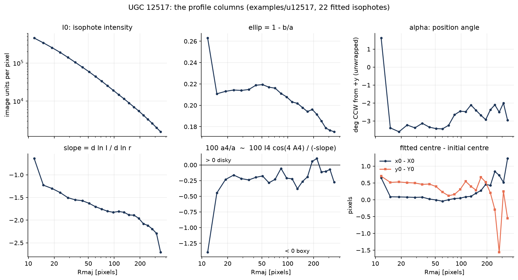
What you can read from it:

• The intensity falls smoothly, with no breaks.
• The ellipticity is about 0.21 out to ~70 pixels (9″), then falls slowly to 0.175: the galaxy is rounder in its outskirts.
• The position angle is constant to within about 1.5°: no isophote twist.
• The slope steepens outwards, as expected for an elliptical galaxy.
• a4/a is within a few tenths of a percent of zero: nearly pure ellipses.
• The centres agree to better than half a pixel inside ~100 pixels, and scatter by up to 1.5 pixels further out, where the galaxy is faint and heavily masked.

The second isophote (11.7 pixels) is also affected by the masked nucleus: its ellipticity and I4 differ from their neighbours.

Plotting conventions

Position angles near 0° and 180°

alpha is an axis direction, so 0° and 180° are the same. A galaxy with its major axis near the image's y axis can jump between ~2° and ~178° from one isophote to the next, although the orientation has barely changed. To plot it, unwrap the angles:

import numpy as np
alpha = np.degrees(np.unwrap(np.radians(2 * p.alpha))) / 2

• Plot the radius on a log axis, or as \(r^{1/4}\) (a de Vaucouleurs law is then a straight line in magnitudes).
• Plot intensities on a log axis, or as surface brightness in magnitudes.

Reading the files

from elliprof import read_profile, read_prf

p = read_profile("u12517.dat")       # pandas DataFrame
print(p.attrs["scale"])              # SCALE= (arcsec/pixel), if given

raw = read_prf("u12517.dat")         # dict: n, scale, params (250 x 12), header

The CSV starts with # comment lines (input, mask, sky, parameters, version, units, and the column names). elliprof reads it back with parse_elliprof_csv:

from elliprof import parse_elliprof_csv
p, meta = parse_elliprof_csv("u12517.csv")    # DataFrame, dict of header lines
print(meta["Sky"], meta["Parameters"])

With another CSV reader, skip the # lines and supply the column names (they are in elliprof.COLUMNS): pandas.read_csv("u12517.csv", comment="#", header=None, names=elliprof.COLUMNS, skipinitialspace=True).