Power spectrum and distance

This page describes, in outline, how an SBF analysis turns a residual image into a distance. None of these steps is performed by ELLIPROF. They are shown so that you can see where ELLIPROF's products are used. For the real procedures, follow the papers listed on History and references, especially Jensen et al. (2015) ("Calibration and Advice") and Cantiello & Blakeslee (2023).

1. Normalise the residual

The fluctuation variance at a point is proportional to the galaxy's brightness there. Dividing the residual by the square root of the model makes the fluctuation amplitude the same everywhere:

\[ r(x, y) = \frac{\text{science} - \text{sky} - \text{model}}{\sqrt{\text{model}}} \]

Point sources, masked regions and the parts of the galaxy that are too faint or too disturbed are excluded, usually by analysing one or more annuli.

2. Take the power spectrum

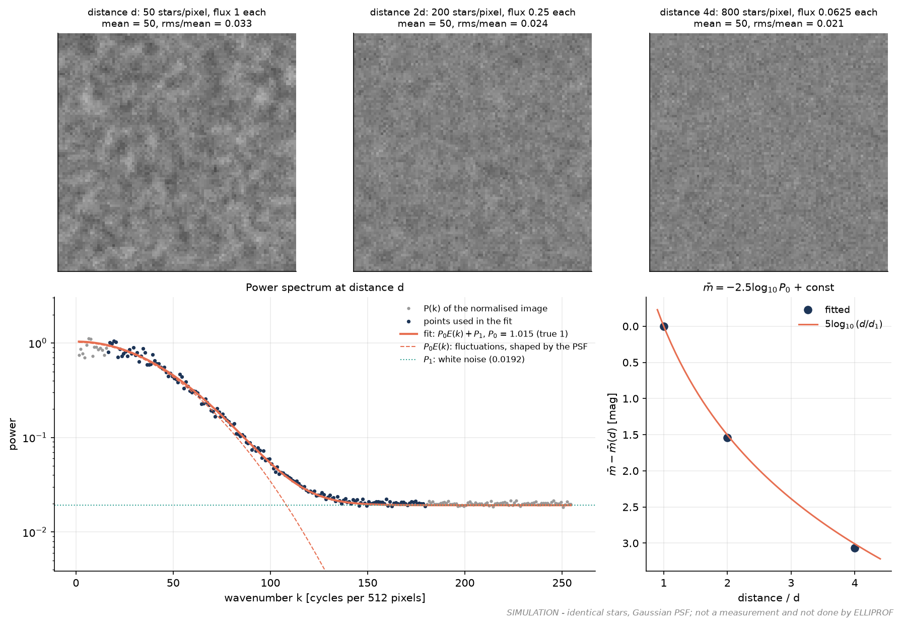
The 2-D Fourier transform of \(r\) is squared, and its power is averaged in rings of constant wavenumber \(k\) to give \(P(k)\).

The fluctuations come from the stars, which are point sources, so in the image they are all blurred by the point-spread function (PSF). Their power spectrum therefore has the shape of the PSF's power spectrum. The noise of the detector and the sky is uncorrelated between pixels, so its power spectrum is flat. Hence

\[ P(k) = P_0\,E(k) + P_1 \]

• \(E(k)\) is the expectation power spectrum: the power spectrum of the PSF, convolved with the power spectrum of the mask (the "window") used in the analysis;
• \(P_0\) is the fluctuation power, what we want;
• \(P_1\) is the white-noise power.

\(P_0\) and \(P_1\) are fitted over a range of \(k\). The lowest wavenumbers are avoided, because residual large-scale structure from an imperfect galaxy model or sky lives there. So are the highest, where the noise dominates.

SIMULATION (identical to the figure on the SBF overview). With a known input, the fit recovers the fluctuation power and the noise level.

3. Correct for sources you did not remove

Globular clusters and background galaxies fainter than the detection limit remain in the image and add their own power, \(P_r\). It is estimated by fitting the luminosity functions of the detected sources and extrapolating below the limit. The stellar fluctuation power is \(P_0 - P_r\). At large distances this correction can be important.

4. Fluctuation magnitude

Because the residual was normalised by √model, \(P_0 - P_r\) is the fluctuation flux, in the image's flux units. With the photometric zeropoint \(m_1\) (the magnitude of one unit of flux),

\[ \bar m = -2.5\log_{10}(P_0 - P_r) + m_1, \]

corrected for Galactic extinction and, for distant galaxies, with a K-correction.

5. Calibration and distance

The absolute fluctuation magnitude \(\bar M\) comes from a calibration, usually a linear relation with galaxy colour, specific to each filter and camera. For example:

• HST/ACS F814W, as a function of \(g - I\) (Blakeslee et al. 2010);
• HST/WFC3-IR F110W and F160W, as a function of \(g - z\) or \(J - H\) (Jensen et al. 2015).

The calibration's zeropoint is tied to galaxies with Cepheid or tip-of-the-red-giant-branch distances (Blakeslee et al. 2021). Then

\[ \mu = \bar m - \bar M, \qquad d = 10^{(\mu + 5)/5}\ \text{pc} = 10^{(\mu - 25)/5}\ \text{Mpc}. \]

Use the calibration that matches your data

\(\bar M\) is not universal. It depends on the filter, the camera, the stellar population (through the colour), and the calibration's zeropoint. A calibration must not be extrapolated beyond the colour range it was derived for (Blakeslee et al. 2010). Quote the calibration you used.

Worked numbers (illustration only)

If a galaxy had \(\bar m = 30.0\) in some band and the calibration gave \(\bar M = -1.5\) at its colour, then \(\mu = 31.5\) and \(d = 10^{(31.5 - 25)/5} = 20\) Mpc. These are round numbers chosen for the arithmetic; they are not a measurement of any galaxy.