SBF workflow and cautions
The whole chain
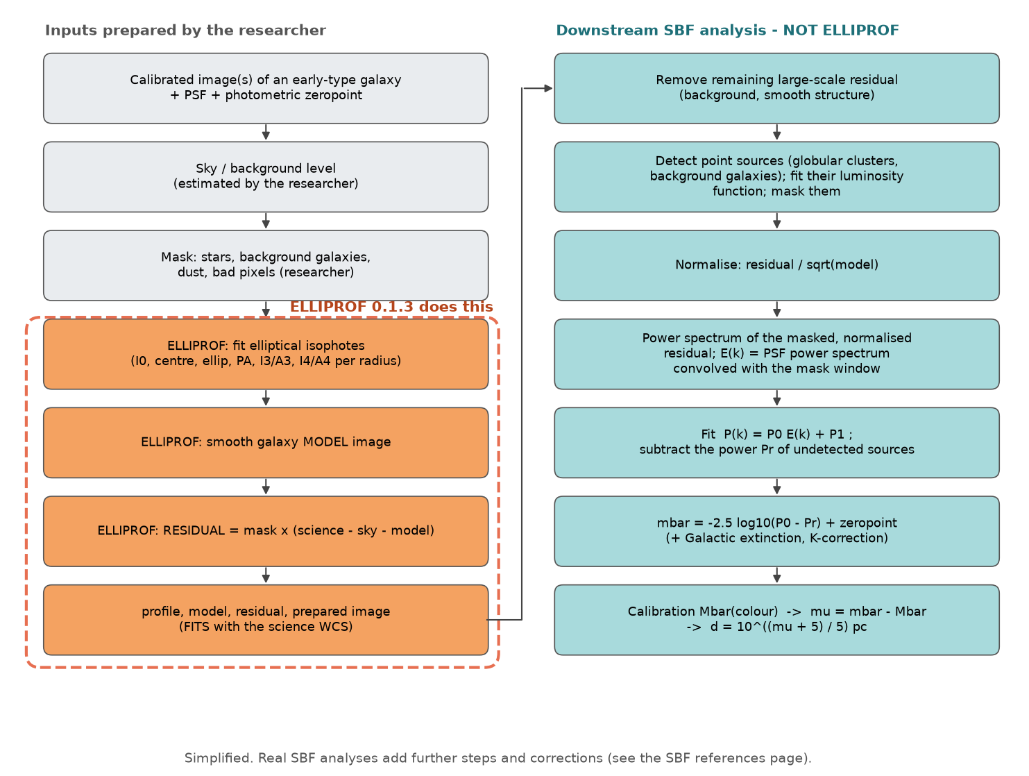
Step by step
| Step | Who does it | Notes |
|---|---|---|
| Reduce and calibrate the images; measure the PSF | researcher | a PSF from stars in the same image or a model; a photometric zeropoint |
| Estimate the sky | researcher | ELLIPROF never estimates it. See Sky and masks |
| Build the mask | researcher | stars, background galaxies, dust, defects |
| Fit isophotes; build the model | ELLIPROF | How ELLIPROF fits a galaxy |
| Write the residual | elliprof | --residual; float32 with the science WCS |
| Remove the remaining large-scale residual | downstream | e.g. smoothing the residual on large scales |
| Detect point sources; fit their luminosity functions; mask them | downstream | globular clusters and background galaxies |
| Normalise by √model; choose the annuli | downstream | |
| Power spectrum; E(k); fit \(P_0\), \(P_1\) | downstream | Power spectrum and distance |
| Subtract the residual-source power \(P_r\) | downstream | from the luminosity-function fits |
| \(\bar m\); extinction and K-correction | downstream | |
| Calibration \(\bar M\)(colour) → \(\mu\) → \(d\) | downstream | filter- and camera-specific |
Cautions
What affects an SBF measurement
- Sky. An error in the sky changes the model and the normalisation. Its effect grows outwards.
- Galaxy model. A poor model leaves large-scale structure in the residual. That adds power at low \(k\), which can be mistaken for fluctuation power if the fit range is not chosen carefully.
- Dust. Dust makes its own "fluctuations" and must be masked. SBF is not reliable in dusty regions.
- Young populations. Recent star formation changes \(\bar M\). The colour calibrations assume old, early-type populations.
- Globular clusters and background galaxies. Undetected sources add power. Their correction depends on the depth of the data and the assumed luminosity functions.
- PSF. \(E(k)\) depends on the PSF. A PSF mismatch biases \(P_0\).
- Noise and depth. The fluctuations must be well above the white-noise floor \(P_1\). Distant galaxies need deep data.
- Calibration. Use the calibration for your filter and camera. Stay inside its colour range, and quote its zeropoint.
Model settings that matter for SBF
- Fit out to where the galaxy is still well above the sky noise, and analyse only the annuli between R0 and R1. Outside that range the model is extrapolated, not fitted.
- Keep the 3rd- and 4th-order terms in the model (the default), and check what they do to the residual; see Harmonics and SBF distances. If you use the 6th order, read its known model limitation.
- Use enough isophotes (
NR) that the model follows the profile smoothly, and enough iterations (NITER) for the parameters to settle. - Mask generously. The residual on masked pixels is 0, so the downstream analysis can use the same mask.
- Check the residual visually and in its power spectrum at low \(k\).
What a result should report
- the images, filter and exposure time;
- the sky level and how it was measured;
- the mask, and how point sources were selected;
- the galaxy-model settings (for ELLIPROF:
R0,R1,NR,RLAW,NITER, the model harmonics, the elliprof version); - the annuli and \(k\) range of the power-spectrum fit;
- \(P_0\), \(P_1\), \(P_r\), \(\bar m\) and their uncertainties;
- the calibration used, \(\bar M\), \(\mu\) and \(d\), with statistical and systematic uncertainties.