A residual for SBF work
This tutorial prepares the input an SBF analysis starts from: a smooth galaxy model and the residual image. It uses UGC 12517 and stops where ELLIPROF's role ends; the later steps of an SBF distance (point-source corrections, the PSF, the power-spectrum fit and a calibration) are described in Workflow. The numbers below are checks of the galaxy model.
1. Fit and write the products
elliprof u12517j.fits \
    --mask u12517j.dmask --sky 3246 \
    X0=567 Y0=562 R0=9 R1=347 NR=23 NITER=10 RMSTAR \
    -o u12517.dat \
    -m u12517.prf --residual u12517_residual.fits
- The model keeps the default 3rd- and 4th-order harmonic terms (see Harmonic analysis).
- The residual is
mask × (science − sky − model): 0 on masked pixels, float32, with the science image's WCS.
2. Look at it
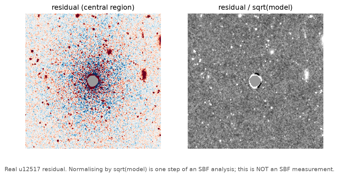
Look for:
- rings or 4-fold patterns: the model does not follow the galaxy.
Try more isophotes (
NR), more iterations (NITER), or check the model harmonics. - a large-scale gradient or offset: the sky is wrong, or the galaxy has structure (dust, disk) that the model cannot describe.
- point sources: globular clusters and background galaxies that the mask did not remove. The downstream analysis must detect them.
3. Check the residual in annuli
In elliptical annuli that follow the galaxy, the median residual should
be a very small fraction of the model. (This table is made by
docs/scripts/residual_checks.py.)
| annulus (a, pixels) | good pixels | median residual | median residual / median model | robust rms of residual/√model |
|---|---|---|---|---|
| 20–40 | 2,986 | −8.1 | −0.0001 | 2.11 |
| 40–80 | 11,935 | −16.5 | −0.0004 | 2.11 |
| 80–160 | 47,785 | 7.8 | +0.0006 | 2.13 |
| 160–320 | 180,849 | 5.0 | +0.0015 | 2.47 |
- The median residual is below 0.2% of the model in every annulus. The model removes the galaxy's smooth light well.
- The scatter of residual/√model (a robust, MAD-based estimate that ignores most unmasked sources) combines photon noise, detector noise, any remaining sources and the stellar fluctuations. Separating these is exactly what the power-spectrum analysis does; the scatter alone is not an SBF measurement.
4. Normalise (downstream, for illustration)
The first downstream step is usually to divide by √model. In Python:
import numpy as np
from astropy.io import fits
from elliprof import load_mask

res = fits.getdata("u12517_residual.fits").astype(float)
model = fits.getdata("u12517.prf").astype(float)
good = load_mask("u12517j.dmask") != 0   # the same mask as the fit

norm = np.full(res.shape, np.nan)
ok = good & (model > 0)
norm[ok] = res[ok] / np.sqrt(model[ok])

hdr = fits.getheader("u12517_residual.fits")   # keeps the WCS
fits.writeto("u12517j_norm.fits", norm.astype(np.float32), hdr, overwrite=True)
Why not just use res != 0?
elliprof sets masked pixels to exactly 0, so res != 0 is nearly the
mask, but not quite. A good pixel can also be exactly 0. In the
UGC 12517 residual, 2 good pixels are exactly 0 (103,404 zeros for
103,402 masked pixels). Use the original mask.
5. Hand over
For the downstream analysis you now have:
| File | Use |
|---|---|
u12517.prf |
normalisation (√model), and the galaxy brightness for colours |
u12517_residual.fits |
the fluctuation image, before large-scale cleaning and point-source masking |
u12517.dat |
the isophote geometry, e.g. to define elliptical annuli |
| the mask | the same pixels to exclude |
Record the elliprof version, the sky, the mask and every fit parameter with your SBF result (see What a result should report).
Next
- Power spectrum and distance: what the downstream analysis does with these files.
- SBF history and references: the papers that describe the full procedures.